roadmap

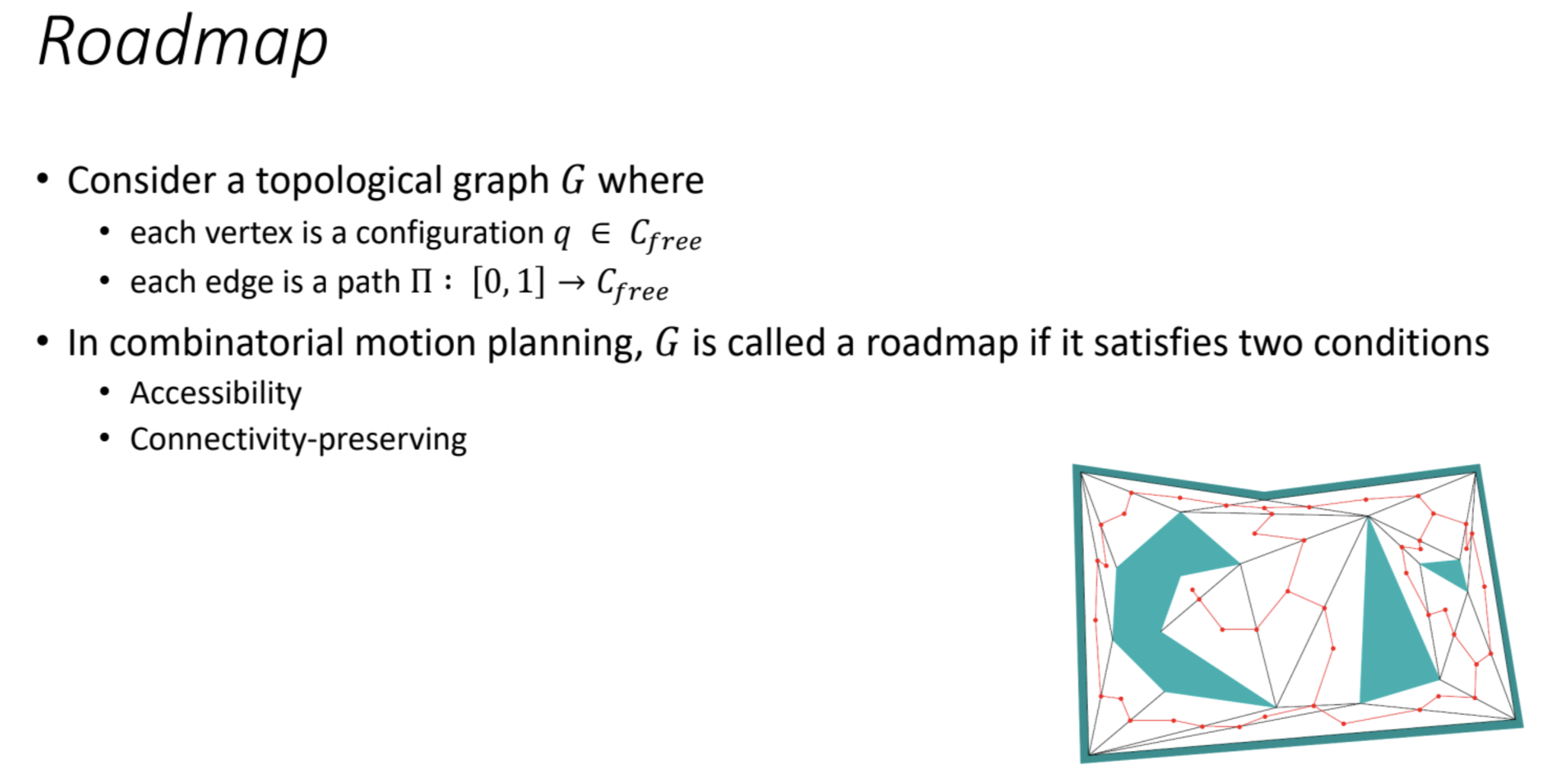
The slide you’ve provided discusses the concept of a "roadmap" in the context of combinatorial motion planning. Here’s an explanation of the key elements:

1. Topological Graph G:

   • A graph $G$ is considered, where:
     • Vertices represent different configurations $q$ that belong to a free configuration space, denoted as $C_{free}$.
     • Edges represent paths $\Pi$ that connect these configurations. Each path is a function from the interval [0, 1] to $C_{free}$, meaning the path continuously maps the interval from the start to the end configuration.

2. Conditions for a Roadmap:
   In combinatorial motion planning, $G$ is termed a "roadmap" if it satisfies two main conditions:

   • Accessibility: The roadmap should allow for all configurations to be accessible, meaning you can navigate from one configuration to another within the configuration space.
   • Connectivity-preserving: The roadmap must maintain connectivity, ensuring that the graph allows continuous paths between configurations without disconnections.

3. Graph Representation:
   The image shows a graphical representation of a roadmap, where configurations are represented as vertices and paths as edges. The diagram illustrates how these paths are arranged and connected to form a topological graph in motion planning.

accessibility refers to the ability to reach or navigate between configurations in the free configuration space, denoted as $C_{\text{free}}$, using the roadmap graph $G$.

To break it down:

1. Configuration Space:

   • A configuration space is a representation of all possible states (positions and orientations) that an object (e.g., a robot or a vehicle) can be in. $C_{\text{free}}$ specifically refers to the subset of that space where no obstacles exist—this is the "free" part of the space.

2. Graph Representation:

   • The roadmap $G$ is a topological graph where each vertex represents a configuration in $C_{\text{free}}$, and each edge represents a continuous path between two configurations.

3. Accessibility in a Roadmap:

   • A roadmap is said to be accessible if, for any configuration in $C_{\text{free}}$, there is a way to move to any other configuration using the paths represented by the edges in the graph. In other words, you should be able to find a path from any starting configuration to a target configuration by following the edges of the roadmap.
   • This means that all configurations in $C_{\text{free}}$ should be "connected" in some way, either directly or indirectly, through paths that represent feasible motions between them.

Key Points of Accessibility:

• Path Availability: Every configuration must have a path that leads to other configurations, meaning there are no isolated vertices or unreachable areas in $C_{\text{free}}$.
• Connectivity: If a configuration is not accessible from another, it implies that some part of the space is disconnected, which would be a failure in the roadmap’s design.

visibility graph

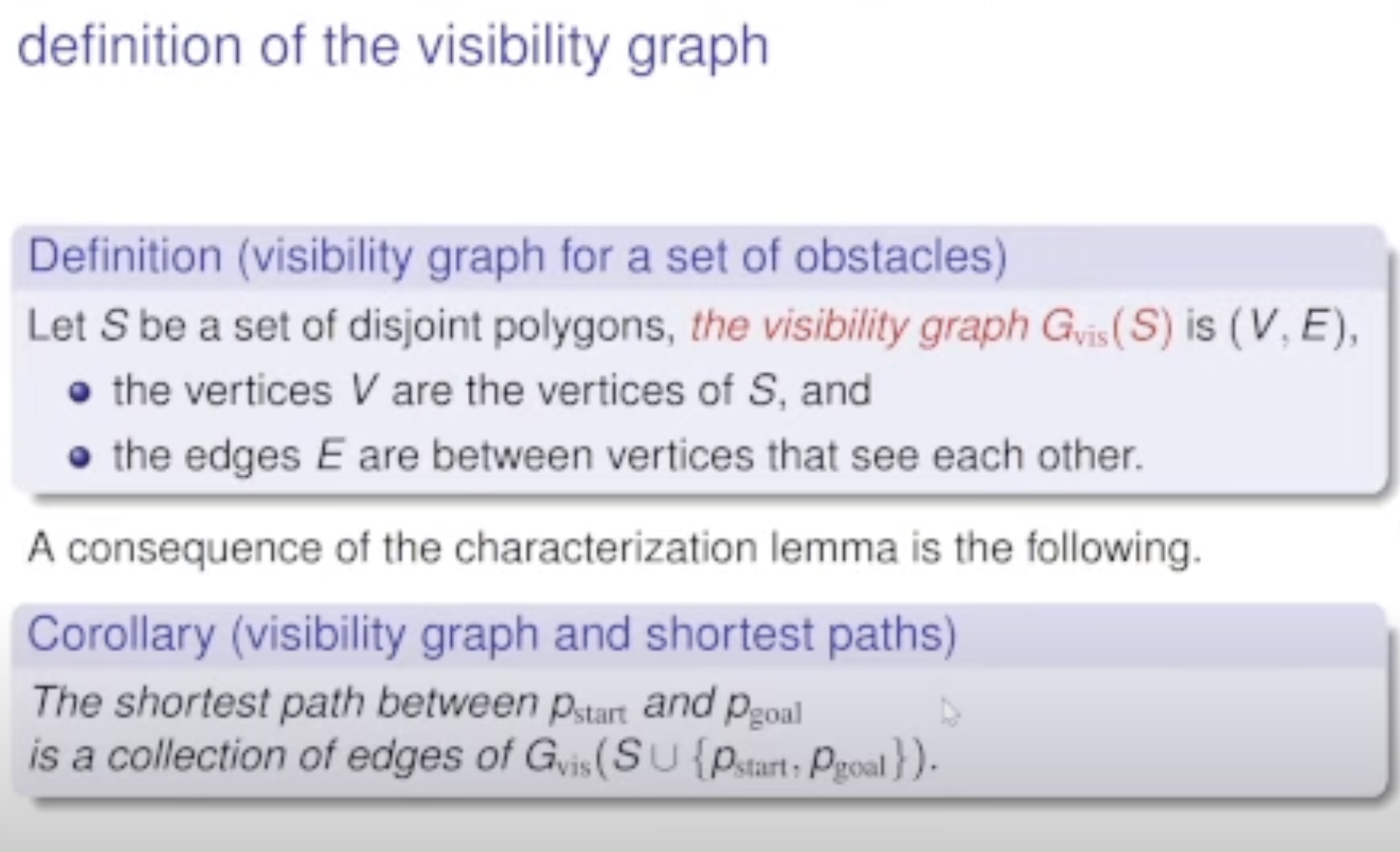
the pic above is not a visibility graph

one animations: https://www.youtube.com/watch?v=rs1t8LxjEW4

https://www.cs.cmu.edu/~motionplanning/lecture/Chap5-RoadMap-Methods_howie.pdf

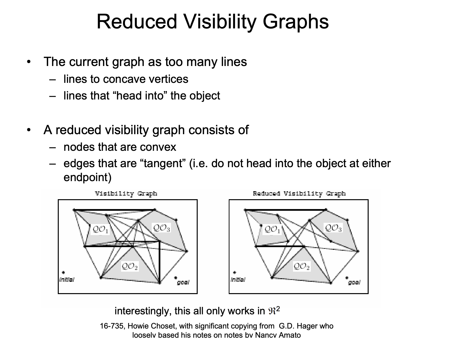
The current graph as too many lines

• lines to concave vertices
• lines that “head into” the object

A reduced visibility graph consists of

• nodes that are convex

• edges that are “tangent” (i.e. do not head into the object at either endpoint)
  What does "convex" mean here?

• Convex vertices: In computational geometry, a convex vertex is a vertex of a polygon where the interior angle is less than 180° (e.g., corners of a rectangle or triangle).

• Convex nodes: In the reduced visibility graph (RVG), nodes are placed at convex vertices of obstacles or critical points in the environment.
  Why convex vertices?

• Convex vertices are “extreme points” that define the outer boundaries of obstacles.

• Paths around obstacles often “hug” these convex vertices to avoid collisions.

• Including only convex vertices reduces the number of nodes compared to a full visibility graph (which includes all obstacle vertices).
  What does “tangent” mean here?

• An edge is tangent if it “grazes”（擦过） an obstacle at its endpoints (nodes) without entering the obstacle’s interior.

• Visually, the edge touches the obstacle only at its endpoints (nodes) and does not intersect the obstacle’s boundary elsewhere.

Why tangent edges?

• Tangent edges ensure that the path stays collision-free while moving between nodes.
• They represent the shortest viable path around obstacles.

Example:

• Suppose two convex nodes (A and B) are on two different obstacles. A tangent edge connects A and B such that the line between them does not penetrate either obstacle.

Key Takeaways

• Nodes = Convex vertices of obstacles.
• Edges = Lines that “hug” obstacles at endpoints (tangent) and are collision-free.
• The RVG is a simplified but powerful tool for efficient path planning.

method 1 use shortest path to make RVG

1. Understand the Context

• What is a Reduced Visibility Graph?
  • A Reduced Visibility Graph is a simplified version of a Visibility Graph, which is used in computational geometry and robotics for path planning.
  • It represents the connections (edges) between points (vertices) in a space where obstacles are present, but with fewer edges than a full visibility graph to reduce complexity.
• Why is it used?
  • It simplifies pathfinding by reducing the number of edges while still maintaining connectivity between critical points.

---

2. Steps to Create a Reduced Visibility Graph

Step 1: Define the Environment

• Represent the environment as a 2D or 3D space with obstacles.
• Obstacles are typically polygons (e.g., rectangles, triangles).
• Identify the start and goal points for pathfinding.

Step 2: Identify Key Points (Vertices)

• Include:
  • All obstacle corners (vertices of polygons).
  • Start and goal points.
• These points will serve as the vertices of the visibility graph.

Step 3: Construct the Full Visibility Graph

• For each pair of vertices, check if they are "visible" to each other:
  • Draw a straight line between the two points.
  • If the line does not intersect any obstacle, they are visible, and an edge is added to the graph.
• Repeat for all pairs of vertices.

Step 4: Reduce the Visibility Graph

• The goal is to remove unnecessary edges while preserving connectivity and the ability to find optimal paths.
• Common reduction techniques:
  1. Remove Redundant Edges:
     • If multiple edges between two vertices are not part of the shortest path, remove them.
  2. Prune Non-Critical Edges:
     • Remove edges that are not part of any shortest path between start and goal.
  3. Merge Parallel Edges:
     • If two edges are nearly parallel and close to each other, merge them into a single edge.
  4. Use Convex Hulls:
     • Simplify the graph by focusing on the convex hull of obstacles, ignoring internal edges.

Step 5: Validate the Reduced Graph

• Ensure the reduced graph still contains all necessary paths:
  • Check that the shortest path between the start and goal is preserved.
  • Verify that no critical connections are lost.

---

3. Algorithms for Reduction

• Dijkstra’s Algorithm or A*:
  • Use these algorithms to identify edges that are part of the shortest path and remove those that are not.
• Edge Pruning:
  • Iterate through all edges and remove those that do not contribute to the shortest path.
• Convex Hull Simplification:
  • Focus on the outer boundaries of obstacles to reduce complexity.

---

4. Example Workflow

• Input:
  • A 2D environment with rectangular obstacles.
  • Start point: (0, 0).
  • Goal point: (10, 10).
• Steps:
  1. Identify all obstacle corners and add them as vertices.
  2. Construct the full visibility graph by connecting all visible pairs of vertices.
  3. Reduce the graph by removing edges that are not part of the shortest path from (0, 0) to (10, 10).
  4. Validate the reduced graph to ensure it still contains the optimal path.

---

way2 use the defininations

Steps to Build an RVG from a VG

(a) Remove Non-Convex Nodes

• Convex vertices are those where the interior angle of the obstacle is < 180°.
• Concave vertices (interior angle > 180°) are removed from the graph.
• Result: Only convex vertices remain as nodes.

(b) Remove Non-Tangent Edges

• For each edge in the VG between two convex nodes, check if it is tangent:
  1. The edge must not "head into" the obstacle at either endpoint.
  2. At each convex node, the edge should align with the obstacle’s boundary (i.e., follow the obstacle’s edge or graze it).
• Remove edges that fail this test.

---

3. Example Workflow

• Input: A VG with nodes at all obstacle vertices (convex and concave).
• Step 1: Delete all concave nodes (e.g., "indentations" in polygons).
• Step 2: For the remaining edges between convex nodes:
  • Check if the edge is tangent to both obstacles at its endpoints.
  • Remove edges that penetrate the obstacle’s interior at either endpoint.
• Output: An RVG with only convex nodes and tangent edges.

4. Tools for Verification

• Visualization: Plot the VG and RVG to confirm tangent edges and convex nodes.
• Collision Checking: Use geometric libraries (e.g., Shapely in Python) to verify edge tangency.
• Path Validation: Ensure shortest paths in the VG are preserved in the RVG.