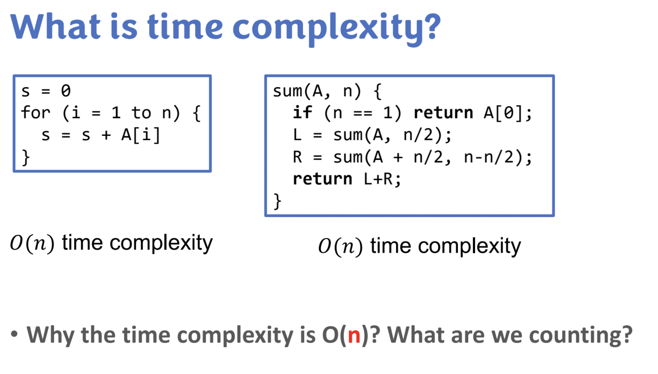
Time complexity is a way to describe how the running time of an algorithm changes relative to the size of its input.

In other words, it answers the question:

“If I make the input bigger, how much longer will this algorithm take to run?”

Key Points:

Input size is usually denoted as n.
Time complexity is often expressed using Big O notation (e.g., O(n), O(log n), O(n²)).
It focuses on the growth rate, not the exact time in seconds.
It helps compare the efficiency of algorithms, especially for large inputs.

Examples:

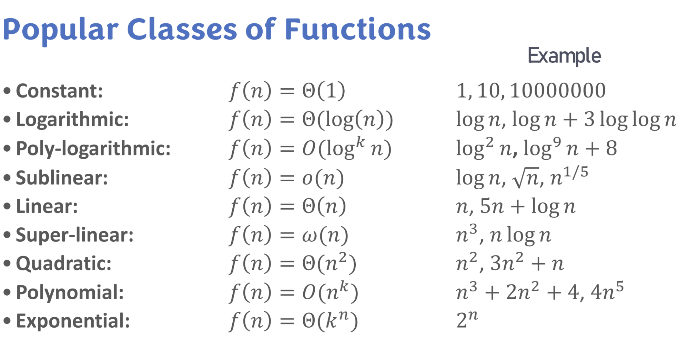
O(1) – constant time: Doesn’t depend on input size (e.g., accessing an array element).
O(n) – linear time: Time grows proportionally with input size (e.g., iterating through a list).
O(n²) – quadratic time: Time grows with the square of the input size (e.g., nested loops).

computation model

Random-Access Machine

Computation Model

A computation model is a simplified, idealized way to understand how an algorithm runs on a computer. It helps us analyze things like time complexity and space complexity without worrying about specific hardware or machine differences.

One of the most common models is the Random-Access Machine (RAM) model.

Random-Access Machine (RAM) Model

The RAM model is a theoretical model that simulates how a real computer works. It’s simple but powerful enough to analyze most standard algorithms.

Key Characteristics:

Instructions: The RAM model executes instructions one at a time — like add, subtract, load, store, compare, branch, etc.
Memory Access: Any memory cell can be accessed in constant time (O(1)), no matter its address — this is what "random access" means.
Memory Structure: The memory is an array of cells, each holding a number or a pointer. There’s no limit on size unless you’re studying space complexity.
Registers: The model has a small number of registers for fast access to data during computation.
No parallelism: It runs one operation at a time (unlike modern CPUs which can be parallel or pipelined).

Why It’s Useful:

It gives us a standard way to measure time complexity.
It avoids hardware-specific details (like cache, I/O, or instruction pipelining), so you can focus on algorithm behavior.

🧠 Example:

Say you have a loop that adds numbers from an array:

sum = 0
for i in range(n):
    sum += arr[i]

In the RAM model:
- Each access to arr[i] takes O(1) time.
- The loop runs n times.
- So, time complexity = O(n).

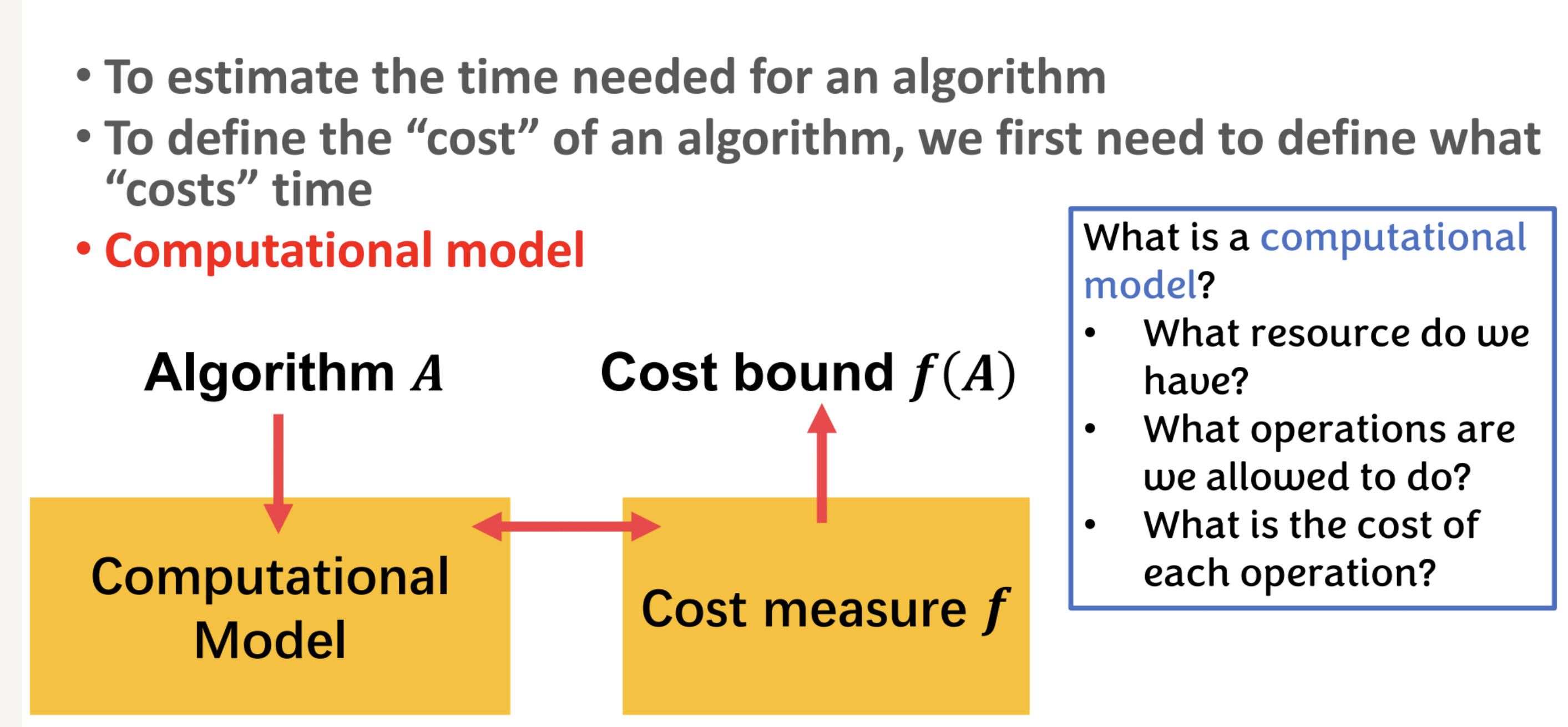
This diagram explains how we analyze the time cost of an algorithm using a computational model. Here’s a breakdown:

🔹 Goal:

To estimate the time needed for an algorithm to run, we need to define what counts as “cost” — and that’s where computational models come in.

🔸 Core Components:

1. Algorithm A

This is the algorithm you want to analyze.

2. Computational Model

This defines how the algorithm runs and what is considered costly.
It answers:
- What resources do we have? (e.g., memory, CPU)
- What operations are allowed? (e.g., add, multiply, read memory)
- What is the cost of each operation? (e.g., is addition O(1)?)

The RAM model is a common computational model where:

Basic operations take constant time (O(1)).
Memory is infinite and accessed in constant time.

3. Cost Measure f

A function that maps the algorithm to a numeric cost — usually how many operations it performs.
Example: If an algorithm runs in linear time, the cost function might be f(A) = O(n).

4. Cost Bound f(A)

The actual time complexity of the algorithm — like O(n), O(log n), or O(n²).
It’s derived from applying the cost measure using the computational model.

🧠 Summary Box (Right Side):

What is a computational model?

What resource do we have?
➜ Like memory, CPU, registers.
What operations can we do?
➜ Can we add, subtract, access arrays, etc.?
What is the cost of each operation?
➜ Constant time? Logarithmic? Depends on model.

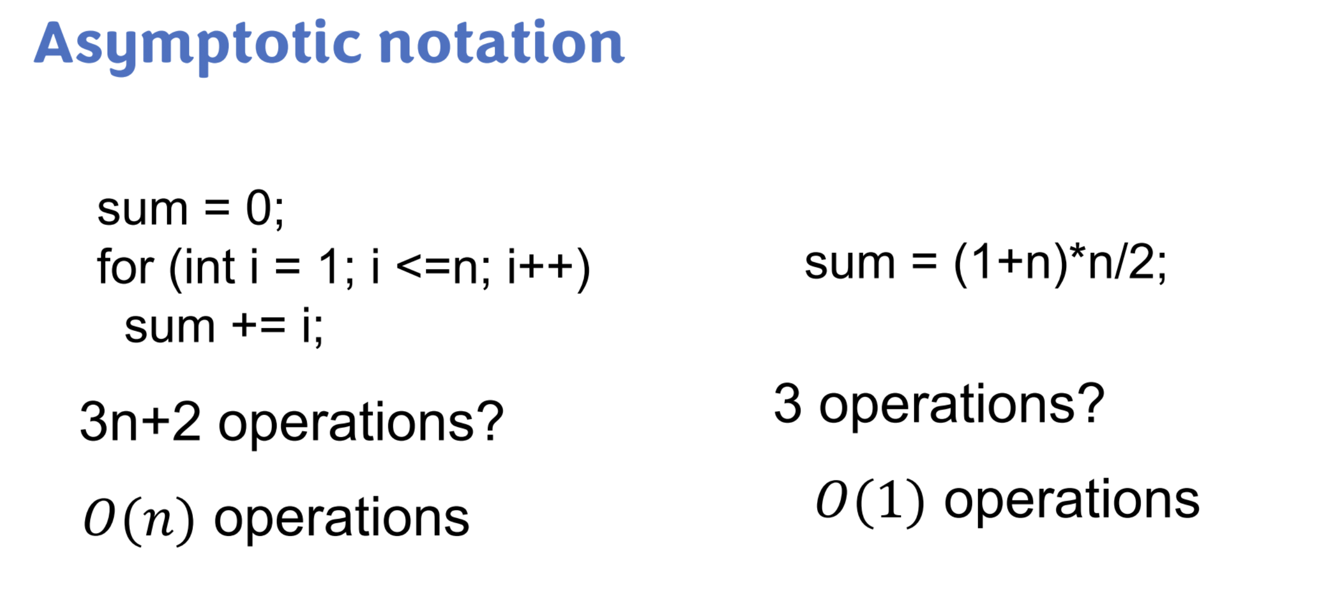
asymptotic analysis

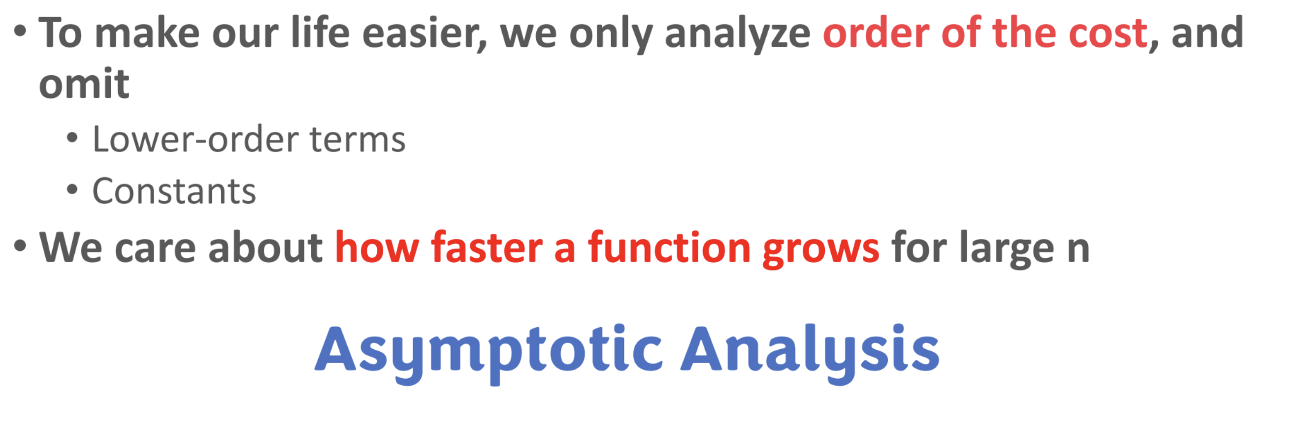
for example:
use O(n) instead of 3n+2

Absolutely! Here’s a clean definition for you:

Big O Notation (𝑂)

Big O is a mathematical notation used to describe the upper bound of an algorithm’s running time (or space use) as a function of input size.

It tells us how the performance of an algorithm scales as the input size grows — focusing on the worst-case scenario.

🔹 Formal Definition:

We say a function

$f(n) = O(g(n))$
if there are constants c > 0 and n₀ ≥ 0 such that:

$$
f(n) \leq c \cdot g(n) \quad \text{for all } n \geq n₀
$$

f(n) is the actual running time.
g(n) is a simpler function (like n, n², log n) that acts as an upper bound.

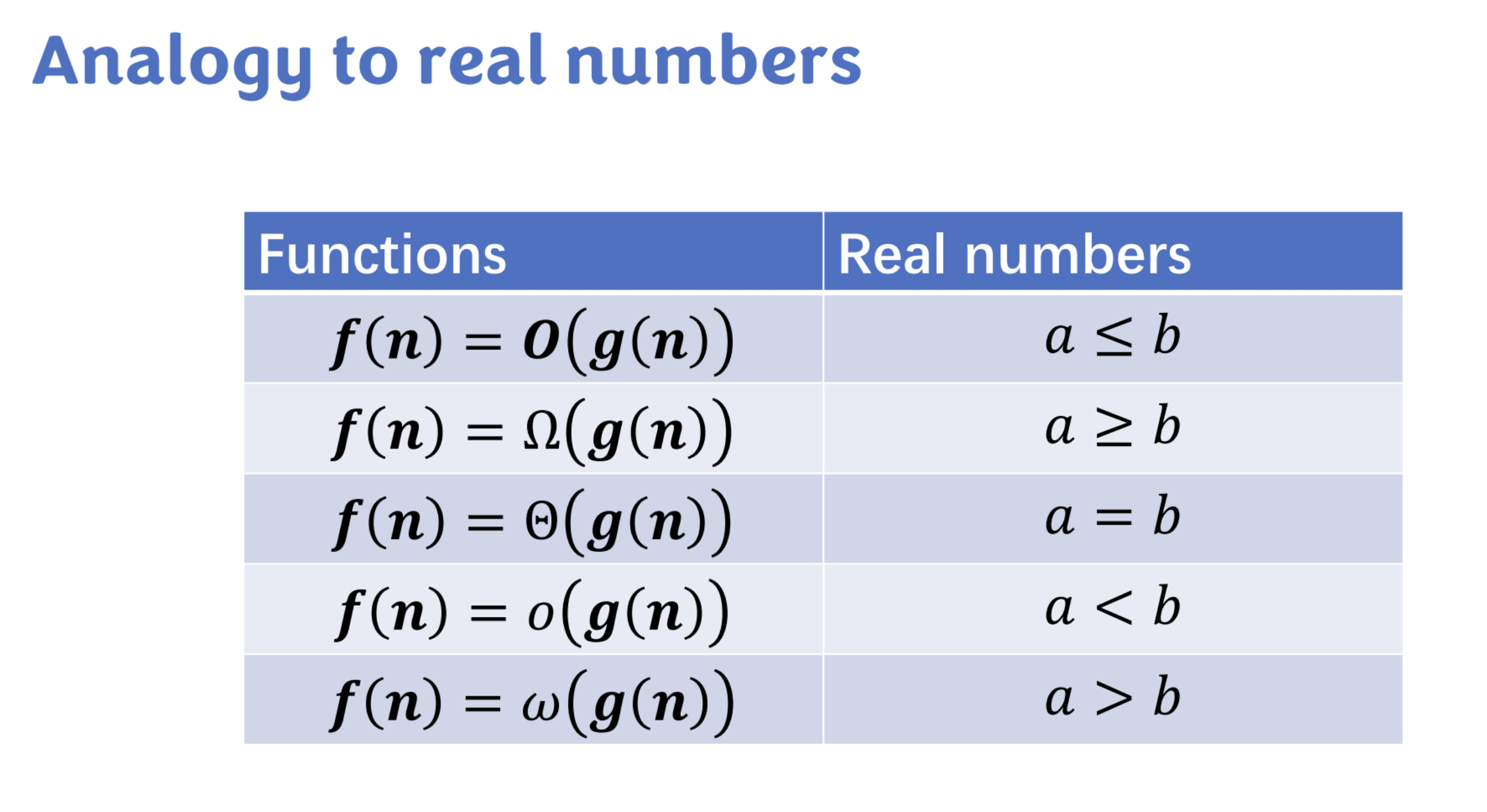
class of the growth

if not sure, take the limit of two functions to compare

cites:

all images are from Yan Gu

algorithm analysis